Section 1.2 solutions

Exercise 1.9

This exercise deals with diferrentiating between recursive and iterative processes by tracing the evaluation of two functions.

Expansion of `(+ 4 5)` using first definition

(define (+ a b)
  (if (= a 0)
      b
      (inc (+ (dec a) b))))

(+ 4 5)
(inc (+ (dec 4) 5))
(inc (+ 3 5))
(inc (inc (+ (dec 3) 5)))
(inc (inc (+ 2 5)))
(inc (inc (inc (+ (dec 2) 5))))
(inc (inc (inc (+ 1 5))))
(inc (inc (inc (inc (+ (dec 1) 5)))))
(inc (inc (inc (inc (+ 0 5)))))
(inc (inc (inc (inc 5))))
(inc (inc (inc 6)))
(inc (inc 7))
(inc 8)
9

As can be seen, there is a chain of deferred inc operations as function is evaluated. Thus, this process is recursive.

Another way to determine that this process is recursive is by observing that the recursive call is nested within another function. The outer function needs to be stored by the interpreter until the inner function returns from the recursive evaluation.

Expansion of `(+ 4 5)` using second definition

(define (+ a b)
  (if (= a 0)
      b
      (+ (dec a) (inc b))))

(+ 4 5)
(+ (dec 4) (inc 5))
(+ 3 6)
(+ (dec 3) (inc 6))
(+ 2 7)
(+ (dec 2) (inc 7))
(+ 1 8)
(+ (dec 1) (inc 8))
(+ 0 9)
9

In this case, there are no deferred operations. The function evaluates exactly to another instance of itself which in turn evaluates to itself till the terminal case. There are no deferred operations to be tracked. Thus, this process is iterative.

Exercise 1.10

This exercise mainly teaches us to interpret procedures into the mathematical functions. For that purpose, we are presented with the Ackermann’s function:-

(define (A x y)
  (cond ((= y 0) 0)
  	((= x 0) (* 2 y))
	((= y 1) 2)
	(else (A (- x 1)
	      	 (A x (- y 1))))))

Evaluating the given expressions, we get

(A 1 10)
; 1024
(A 2 4)
; 65536
(A 3 3)
; 65536

Mathematical definition of `(A 0 n)`

Let us evaluate (A 0 n) for various arguments

(define (f n) (A 0 n))
; f
(f 0)
; 0
(f 1)
; 2
(f 2)
; 4
(f 3)
; 6
(f 4)
; 8
(f 5)
; 10

As can be seen, (f n) evaluates to $2n$ . As we run through the function definition, when (= x 0) evaluates to #t, the Ackermann’s function evaluates to (* 2 y) which is the value we see.

Mathematical definition of `(A 1 n)`

Let us evaluate (A 1 n) for various arguments

(define (g n) (A 1 n))
; g
(g 0)
; 0
(g 1)
; 2
(g 2)
; 4
(g 3)
; 8
(g 4)
; 16
(g 5)
; 32

As can be seen, with the exception of when n is 0, (g n) evaluates to $2^n$ . To see why this is the case, we run through the Ackermann’s function evaluation

(A 1 n)
(A (- 1 1) (A (1 (- n 1))))
(A 0 (A (1 (- n 1))))
(* 2 (A 1 (- n 1)))

...

We can see a series developing. $A(1,n) = 2 \times A(1,n-1)$ in infix notation. The evaluation expands till the terminal case (= n 1) which evaluates to 2. Thus, we multiply 2 with itself n times to get $n^2$

Mathematical definition of `(A 2 n)`

Evaluating (A 2 n) for various arguments, we get

(define (h n) (A 2 n))
; h
(h 0)
; 0
(h 1)
; 2
(h 2)
; 4
(h 3)
; 16
(h 4)
; 65536

Its not clear what is going on immediately. But the expansion of evaluation gives us a clue,

(A 2 n)
(A (- 2 1) (A (2 (- n 1))))
(A 1 (A (2 (- n 1))))

...

Combining with the definition of (A 1 n), we get the relation $A(2,n) = 2^{A(2,n-1)}$ . Expanding down to the terminal case of (= n 1), we see that 2 is powered with itself n times. This can also be written using Knuth’s up-arrow notation as $2\uparrow\uparrow2$ .

Exercise 1.11

This exercise introduces to us the method of solving the same problem using recursive and iterative processes. We have a function similar to Fibonacci series,

$f(n) = \begin{cases} n & n < 3 \\ f(n-1)+2f(n-2)+3f(n-3) & otherwise \end{cases}$

Recursive process

The recursive process can be written simply using the definition.

(define (f n)
(if (< n 3) n
    (+ (f (- n 1))
       (* 2 (f (- n 2)))
       (* 3 (f (- n 3))))))
; f

; Test cases:-
(f 0)
; 0
(f 1)
; 1
(f 2)
; 2
(f 3)
; 4
(f 4)
; 11
(f 5)
; 25
(f 10)
; 1892

Iterative process

The iterative process can be written by using transformations applied on a series of integers similar to the method used for computing Fibonacci series iteratively. Let us initilize $a=f(2)=2$ , $b=f(1)=1$ and $c=f(0)=0$ . We can apply simultaneous transformations.

$\begin{align} a &\leftarrow a+2b+3c \\ b &\leftarrow a \\ c &\leftarrow b \end{align}$

Once the transformations are applied n number of times, c would evaluate to $f(n)$ .

(define (f-iter a b c count)
        (if (= count 0) c
            (f-iter (+ a (* 2 b) (* 3 c)) a b (- count 1))))
; f-iter
 
(define (f n) (f-iter 2 1 0 n))
; f
 
; Test cases:-
(f 0)
; 0
(f 1)
; 1
(f 2)
; 2
(f 3)
; 4
(f 4)
; 11
(f 5)
; 25
(f 10)
; 1892
(f 100)
; 11937765839880230562825561449279733086

The iterative process is more powerful since it can take significantly smaller time in the order of $O(n)$ to compute the result as opposed to the recursive process which takes $O(f(n))$ time to compute.

Exercise 1.12

This exercise makes us write a procedure which evaluates the elements in a Pascal’s triangle using a recursive process. We use the coordinate system below.

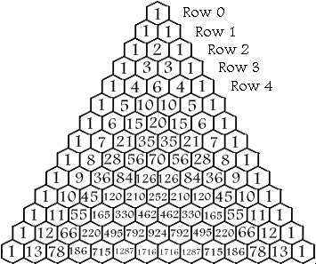
We can define the pascal function at any row and column as such:-

$p(r,c) = \begin{cases} 1 & \text{c=0 or c=r}\\ p(r-1,c) + p(r-1,c-1) & otherwise \end{cases}$

(define (pascal row col)
(if (or (= col 0) (= col row)) 1
    (+ (pascal (- row 1) col)
       (pascal (- row 1) (- col 1)))))
; pascal

; Test cases:-
(pascal 0 0)
; 1
(pascal 100 100)
; 1
(pascal 13 6)
; 1716
(pascal 9 4)
; 126

Exercise 1.13

This exercise wants us to prove that $Fib(n)$ is the closest integer to $\phi^n/\sqrt{5}$ where $\phi=(1+\sqrt{5})/2$ . Let us derive this using the hints given.

Firstly, we are told to prove that

$Fib(n)=(\phi^n-\psi^n)/\sqrt{5}$

where $\psi=(1-\sqrt{5})/2$ . We are also given that $\phi^2=\phi+1$ and $\psi^2=\psi+1$ .

Let us use mathematical induction to prove the relation.

Base case

Left-hand side:-

$\begin{align}Fib(0) &= 0 \\ Fib(1) &= 1 \\ Fib(2) &= Fib(0)+Fib(1)=1\end{align}$

Right-hand side:-

n = 0

$\begin{align}(\phi^n-\psi^n)/\sqrt{5} &= (\phi^0-\psi^0)/\sqrt{5} \\ &= (1-1)/\sqrt{5} \\ &= 0/\sqrt{5} \\ &= 0\end{align}$

n = 1

$\begin{align}(\phi^n-\psi^n)/\sqrt{5} &= (\phi^1-\psi^1)/\sqrt{5} \\ &= ((1+\sqrt{5})/2-(1-\sqrt{5})/2)/\sqrt{5} \\ &= ((2\sqrt{5})/2)/\sqrt{5} \\ &= \sqrt{5}/\sqrt{5} \\ &= 1\end{align}$

n = 2

$\begin{align}(\phi^n-\psi^n)/\sqrt{5} &= (\phi^2-\psi^2)/\sqrt{5} \\ &= ((\phi+1)-(\psi+1))/\sqrt{5} \\ &= (\phi-\psi)/\sqrt{5} \\ &= 1\end{align}$

Inductive step

Let us assume that the following relations hold true,

$\begin{align} Fib(n) &= (\phi^n-\psi^n)/\sqrt{5} \\ Fib(n-1) &= (\phi^{n-1}-\psi^{n-1})/\sqrt{5}\end{align}$

We need to prove that the assumptions lead to

$Fib(n+1) = (\phi^{n+1}-\psi^{n+1})/\sqrt{5}$

From definition,

$\begin{align}Fib(n+1) &= Fib(n)+Fib(n-1) \\ &= (\phi^n-\psi^n)/\sqrt{5} + (\phi^{n-1}-\psi^{n-1})/\sqrt{5} \\ &= (\phi^n+\phi^{n-1})/\sqrt{5} - (\psi^n+\psi^{n-1})/\sqrt{5} \\ &= (\phi^{n-1}(\phi+1))/\sqrt{5} - (\psi^{n-1}(\psi+1))/\sqrt{5} \\ &= (\phi^{n-1}\phi^2)/\sqrt{5} - (\psi^{n-1}\psi^2)/\sqrt{5} \\ &= (\phi^{n+1}-\psi^{n+1})/\sqrt{5} \end{align}$

Hence, we have proven the relation.

Original problem

Going back to the original problem, we can reformulate it to say that we need to prove $\|Fib(n) - \phi^n/\sqrt{5}\| <= 1/2$ .

From the inductive proof above, we can see that $Fib(n)-\phi^n/\sqrt{5} = \psi^n/\sqrt{5}$ .

Thus, we need to prove $\|\phi^n/\sqrt{5}\| <= 1/2$ or $\|\phi^n\| <= \sqrt{5}/2$ .

We have $\phi = (1-\sqrt{5})/2 \approx -0.618034$ and $\sqrt{5}/2 \approx 1.118034$ .

Since $\|\phi\|<1$ , we have $\|\phi^n\|<1$ where n is any positive integer in $Fib(n)$ .

We can safely say that

$\|Fib(n) - \phi^n/\sqrt{5}\| <= 1/2$

Thus, Fib(n) is the closest integer to $\phi^n/\sqrt{5}$ .

Exercise 1.14

This exercise tasks us with understanding the growth of a recursive process. We are told to draw the tree illustrating the process generated by the given procedure (count-change 11).

(define (count-change amount)
  (cc amount 5))

(define (cc amount kinds-of-coins)
  (cond ((= amount 0) 1)
        ((or (< amount 0) 
             (= kinds-of-coins 0)) 
         0)
        (else 
         (+ (cc amount (- kinds-of-coins 1))
            (cc (- amount (first-denomination 
                           kinds-of-coins))
                kinds-of-coins)))))

(define (first-denomination kinds-of-coins)
  (cond ((= kinds-of-coins 1) 1)
        ((= kinds-of-coins 2) 5)
        ((= kinds-of-coins 3) 10)
        ((= kinds-of-coins 4) 25)
        ((= kinds-of-coins 5) 50)))

The graph obtained is as follows (click to enlarge):-

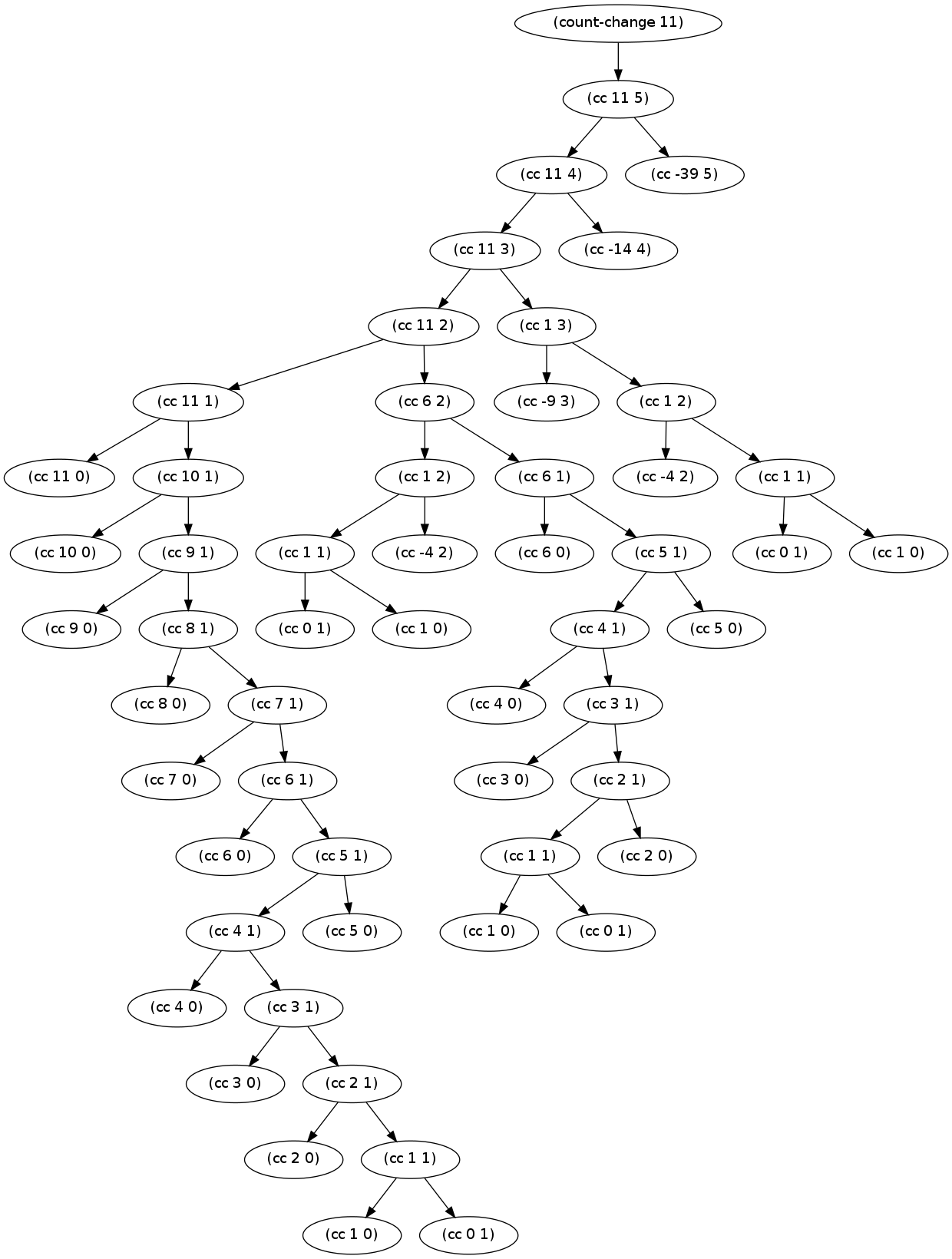
Note:- The Python code used to generate this tree is found here

Complexity of procedure

For the purpose of simplicity, let us denote n as the total amount and m as the number of types of coins(denominations).

Space Complexity: The space complexity of the procedure is fairly straight forward. The maximum space taken by the solution occurs when the most depth is reached. The longest depth can be reached by first taking the branch where kinds-of-coins is reduced to 1 followed by reducing the amount by the smallest denomination of 1. This results in a space complexity of $O(n+m)$ . Since m is usually much smaller than n, we get an asymptotic space complexity of $O(n)$ .

Time Complexity: The time complexity can be determined by building up from simpler cases. Thanks to Bill the Lizard’s post here.

We start with a simple case whereupon we have no coins, ie. we call (cc amount 0). In this case, we get the following graph:-

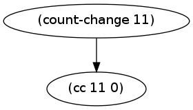
A simple case where we have only one branch yielding time complexity $O(1)$ .

Next, we move to one type of coin invoking (cc amount 1). To determine its time complexity, we look at the process generated for that case:-

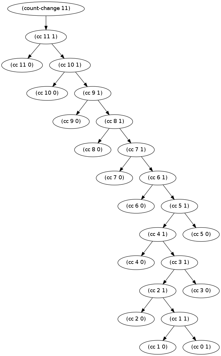
Using the same notation as in space complexity, we can see that in this case, the number of steps taken is given by calling (cc n 1) $n+1$ times with successively smaller values which results in (cc amount 0) given above being called n times, yielding a time of $2n+1$ and time complexity of $O(n)$ .

We next look at two types of coins invoking (cc amount 2). We once again look at the process generated for this case.

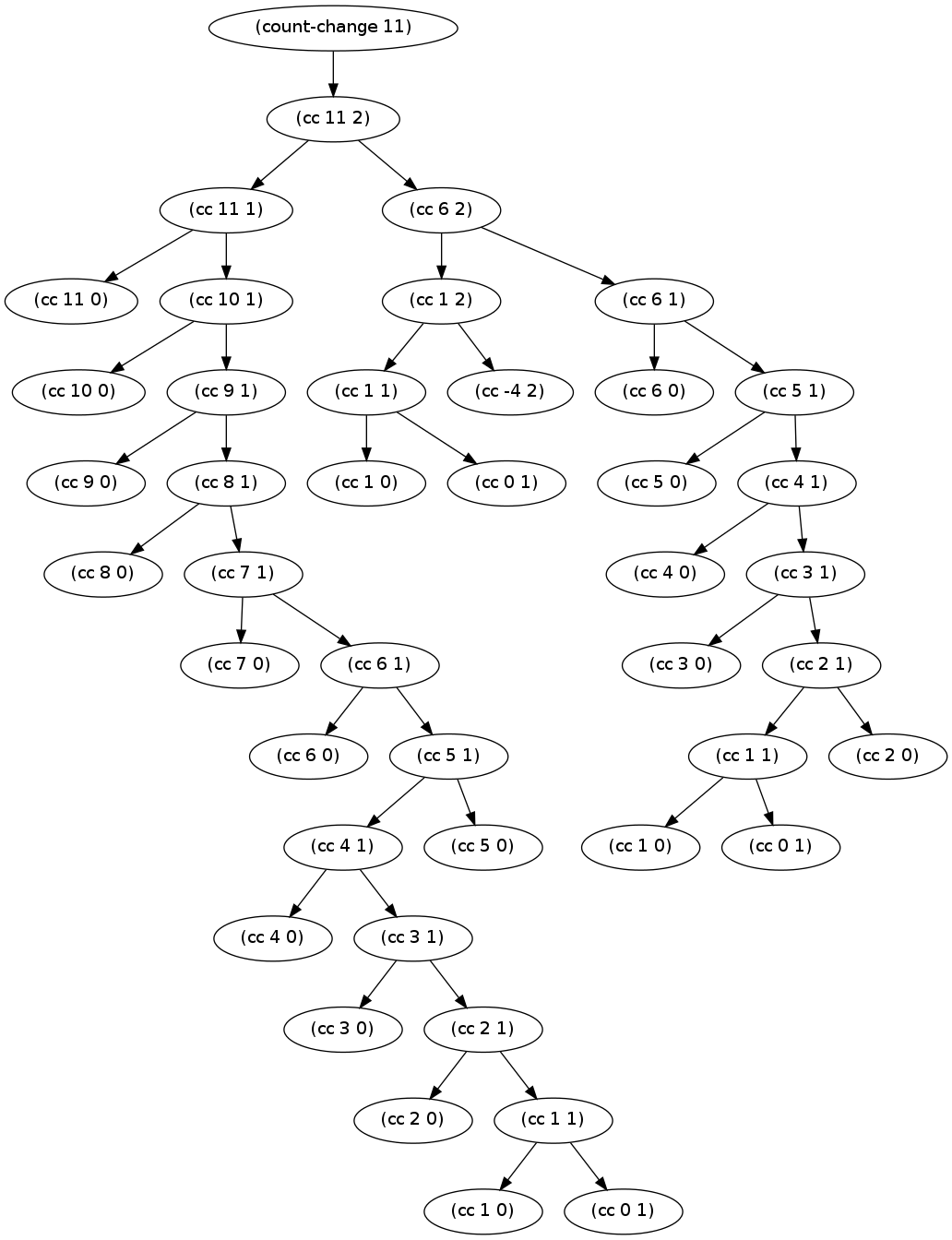
We can see the main path calling (cc n 2) gets called $n/5$ times because of the second denomination of 5 cents. Each node in this path each calls its own (cc n 1) sub-process. Summing them up, we obtain a sum for total time, $(2n+1) + (2(n-5)+1) + (2(n-10)+1) + ...$ . The number of terms in this summation is $n/5$ yielding a time complexity of $O(n^2)$ .

As such, we can see a pattern building up. Since we have five types of coins ultimately, we end up with a final time complexity for (cc amount 5) to be $O(n^5)$ .

Exercise 1.15

As with previous case, we try to analyse the complexity of the following function:-

(define (cube x) (* x x x))
(define (p x) (- (* 3 x) (* 4 (cube x))))
(define (sine angle)
   (if (not (> (abs angle) 0.1))
       angle
       (p (sine (/ angle 3.0)))))

To get the number of times procedure p is applied in evaluating (sine 12.15), we look at its expansion:-

(sine 12.15)
(p (sine (/ 12.15 3.0)))
(p (sine 4.05))
(p (p (sine (/ 4.05 3.0))))
(p (p (sine 1.35)))
(p (p (p (sine (/ 1.35 3.0)))))
(p (p (p (sine 0.45))))
(p (p (p (p (sine (/ 0.45 3.0))))))
(p (p (p (p (sine 0.15)))))
(p (p (p (p (p (sine (/ 0.15 3.0)))))))
(p (p (p (p (p (sine 0.05))))))
(p (p (p (p (p 0.05)))))
(p (p (p (p 0.1495))))
(p (p (p 0.4351)))
(p (p 0.9758))
(p -0.7896)
-0.3998

From the above, we can see that the procedure p is applied 5 times.

Order of growth

The time and space complexity should have the same order in this case because we do not see any branches in the evaluation tree.

As we can see, the number of steps taken by the evaluation of (sine a) increases by one when a is tripled. This hints at a logarithmic growth of $O(log n)$ for both time and space complexity.

Exercise 1.16

This exercise tasks us with writing the given fast-exponentiation function with a procedure utilizing iterative process. It also introduces the concept of a loop invariant. In this case, we use a accummulator variable a which starts at 1 and evaluates to $b^n$ at the end of the iteration. Similar to the rule provided for odd and even powers, we make a new rule such that $ab^n$ does not vary between successive iterations.

$ab^n = \begin{cases} (ab)b^{n-1} & \text{if n is odd} \\ a(b^2)^{n/2} & \text{if n is even} \end{cases}$

We write the procedure in scheme.

(define (fast-expt b n)
  (fast-expt-iter b n 1))
; fast-expt

(define (fast-expt-iter b n a)
  (cond ((= n 0) a)
        ((even? n)
         (fast-expt-iter (square b) (/ n 2) a))
        (else
         (fast-expt-iter b (- n 1) (* a b)))))
; fast-expt-iter

(define (even? n)
  (= (remainder n 2) 0))
; remainder

; Test cases:-
(fast-expt 2 2)
; 4
(fast-expt 5 5)
; 3215
(fast-expt 1.5 10)
; 57.6650390625

Exercise 1.17

This exercise tasks us with writing fast integer multiplication using a method similar to fast exponentiation presented in this section.

$ab = \begin{cases} a + a(b-1) & \text{if b is odd} \\ 2a(b/2) & \text{if b is even} \end{cases}$

Writing new helper functions halve and double, we have

(define (fast-mult a b)
  (cond ((= b 0) 0)
        ((= b 1) a)
        ((even? b) 
         (double (fast-mult a (halve b))))
        (else 
         (+ a (fast-mult a (- b 1))))))
; fast-mult

(define (even? n)
  (= (remainder n 2) 0))
; even?

(define (double n)
  (* n 2))
; double

(define (halve n)
  (/ n 2))
; halve

; Test cases:-
(fast-mult 5 1)
; 5
(fast-mult 113 135)
; 15255
(fast-mult 23 76)
; 1748

Exercise 1.18

In this exercise, we extend the solutions from the previous two exercises to create an iterative process for computing the multiplication of two numbers. In this case, we use an accummulator variable p to hold the intermediate product. We get an invariant of $p + ab$ .

$p + ab = \begin{cases} (p+a)+a(b-1) & \text{if b is odd} \\ p+(2a)(b/2) & \text{if b is even} \end{cases}$

(define (fast-mult a b)
  (fast-mult-iter a b 0))
; fast-mult

(define (fast-mult-iter a b p)
  (cond ((= b 0) p)
        ((even? b)
         (fast-mult-iter (double a) (halve b) a))
        (else
         (fast-mult-iter a (- b 1) (+ p b)))))
; fast-mult-iter

(define (fast-mult a b)
  (cond ((= b 0) 0)
        ((= b 1) a)
        ((even? b) 
         (double (fast-mult a (halve b))))
        (else 
         (+ a (fast-mult a (- b 1))))))
; fast-mult

(define (even? n)
  (= (remainder n 2) 0))
; even?

(define (double n)
  (* n 2))
; double

(define (halve n)
  (/ n 2))
; halve

; Test cases:-
(fast-mult 5 1)
; 5
(fast-mult 113 135)
; 15255
(fast-mult 23 76)
; 1748

Exercise 1.19

In this interesting exercise, we are told to extend the $O(log(n))$ solutions developed in the previous exercises to the computation of the Fibonacci series. To help with that, we develop a generic transformation $T_{pq}$ ,

$\begin{align}a &\leftarrow (p+q)a + qb \\ b &\leftarrow qa + pb\end{align}$

wherein, $T_{01}$ is the special case denoting one step of transformation in generating Fibonacci series. To accelerate this process, let us apply $T_{pq}$ twice to obtain a compact transformation $T_{p'q'}$ that does two steps in one step.

$\begin{align}a_1 &\leftarrow (p+q)a + qb \\ b_1 &\leftarrow qa + p \\ a_2 &\leftarrow (p+q)a_1 + qb_1 \\ &\leftarrow (p+q)[(p+q)a+qb]+q(qa+pb) \\ &\leftarrow (p^2+2pq+q^2)a+(pq+q^2)b+(q^2)a+(pq)b \\ &\leftarrow (p^2+2pq+2q^2)a+(2pq+p^2)b \\ b_2 &\leftarrow qa_1 + pb_1 \\ &\leftarrow q[(p+q)a+qb]+p(qa+pb) \\ &\leftarrow (pq+q^2)a+(q^2)b+(pq)a+(p^2)b \\ &\leftarrow (q^2+2pq)a+(p^2+q^2)b\end{align}$

Ultimately, we obtain $p'=p^2+q^2$ and $q'=q^2+2pq$ .

Substituting it into the provided function template, we get the following code which computes $Fib(n)$ in $O(log(n))$ time.

(define (fib n)
  (fib-iter 1 0 0 1 n))

(define (fib-iter a b p q count)
  (cond ((= count 0) 
         b)
        ((even? count)
         (fib-iter a
                   b
                   (+ (square p) (square q))  ;compute p'
                   (+ (square q) (* 2 p q))   ;compute q'
                   (/ count 2)))
        (else 
         (fib-iter (+ (* b q) 
                      (* a q) 
                      (* a p))
                   (+ (* b p) 
                      (* a q))
                   p
                   q
                   (- count 1)))))

; Test cases:-
(fib 0)
; 0
(fib 1)
; 1
(fib 2)
; 1
(fib 3)
; 2
(fib 4)
; 3
(fib 10)
; 55
(fib 100)
; 354224848179261915075

Exercise 1.20

In this exercise, we revisit the applicative and normal-order evaluation strategies presented in Section 1.1 to trace the given function and determine how many times remainder is called.

(define (gcd a b)
  (if (= b 0)
      a
      (gcd b (remainder a b))))

Normal-order evaluation

In normal-order evaluation, we fully expand first before evaluating.

(gcd 206 40)

(if (= 40 0)
    206
	(gcd 40 (remainder 206 40)))

(gcd 40 (remainder 206 40))

(if (= (remainder 206 40) 0)
    40
    (gcd (remainder 206 40) (remainder 40 (remainder 206 40))))

; 1 evaluation (remainder 206 40) => 6
(if (= 6 0)
    40
    (gcd (remainder 206 40) (remainder 40 (remainder 206 40))))
	
(gcd (remainder 206 40) (remainder 40 (remainder 206 40)))

(if (= (remainder 40 (remainder 206 40)) 0)
    (remainder 206 40)
    (gcd (remainder 40 (remainder 206 40))
         (remainder (remainder 206 40)
                    (remainder 40 (remainder 206 40)))))

; 2 evaluations (remainder 40 (remainder 206 40))
;            => (remainder 40 6) => 4
(if (= 4 0)
    (remainder 206 40)
    (gcd (remainder 40 (remainder 206 40))
         (remainder (remainder 206 40)
                    (remainder 40 (remainder 206 40)))))

(gcd (remainder 40 (remainder 206 40))
     (remainder (remainder 206 40)
                (remainder 40 (remainder 206 40))))

(if (= (remainder (remainder 206 40)
                  (remainder 40 (remainder 206 40))) 0)
    (remainder (remainder 206 40)
               (remainder 40 (remainder 206 40)))
    (gcd (remainder (remainder 206 40)
                    (remainder 40 (remainder 206 40)))
         (remainder (remainder 40 (remainder 206 40))
                    (remainder (remainder 206 40)
                               (remainder 40 (remainder 206 40))))))

; 4 evaluations (remainder (remainder 206 40)
;                          (remainder 40 (remainder 206 40)))
;            => (remainder 6 4) => 2
(if (= 2 0)
    (remainder (remainder 206 40)
               (remainder 40 (remainder 206 40)))
    (gcd (remainder (remainder 206 40)
                    (remainder 40 (remainder 206 40)))
         (remainder (remainder 40 (remainder 206 40))
                    (remainder (remainder 206 40)
                               (remainder 40 (remainder 206 40))))))

(gcd (remainder (remainder 206 40)
                (remainder 40 (remainder 206 40)))
     (remainder (remainder 40 (remainder 206 40))
                (remainder (remainder 206 40)
                           (remainder 40 (remainder 206 40)))))

(if (= (remainder (remainder 40 (remainder 206 40))
                  (remainder (remainder 206 40)
                             (remainder 40 (remainder 206 40)))) 0)
    (remainder (remainder 206 40)
               (remainder 40 (remainder 206 40)))
    (gcd (remainder (remainder 40 (remainder 206 40))
                    (remainder (remainder 206 40)
                               (remainder 40 (remainder 206 40))))
         (remainder (remainder (remainder 206 40)
                               (remainder 40 (remainder 206 40)))
                    (remainder (remainder 40 (remainder 206 40))
                               (remainder (remainder 206 40)
                                          (remainder 40
                                                     (remainder 206 40)))))))

; 7 evaluations (remainder (remainder 40 (remainder 206 40))
;                          (remainder (remainder 206 40)
;                                     (remainder 40 (remainder 206 40))))
;            => (remainder 4 2) => 0
(if (= 0 0) 
    (remainder (remainder 206 40)
               (remainder 40 (remainder 206 40)))
    (gcd (remainder (remainder 40 (remainder 206 40))
                    (remainder (remainder 206 40)
                               (remainder 40 (remainder 206 40))))
         (remainder (remainder (remainder 206 40)
                               (remainder 40 (remainder 206 40)))
                    (remainder (remainder 40 (remainder 206 40))
                               (remainder (remainder 206 40)
                                          (remainder 40
                                                     (remainder 206
                                                                40)))))))

(remainder (remainder 206 40)
           (remainder 40 (remainder 206 40)))

; 4 evaluations
2

As can be seen, the overly long evaluation chain evaluates remainder 18 times.

Applicative-order evaluation

In applicative order evaluation, we evaluate available sub-expressions before expanding.

(gcd 206 40)

(if (= 40 0)
    206
    (gcd 40 (remainder 206 40)))

(gcd 40 (remainder 206 40))

; 1 evaluation
(gcd 40 6)

(if (= 6 0)
    40
    (gcd 6 (remainder 40 6)))

(gcd 6 (remainder 40 6))

; 1 evaluation
(gcd 6 4)

(if (= 4 0)
    6
    (gcd 4 (remainder 6 4)))

(gcd 4 (remainder 6 4))

; 1 evaluation
(gcd 4 2)

(if (= 2 0)
    4
    (gcd 2 (remainder 4 2)))

(gcd 2 (remainder 4 2))

; 1 evaluation
(gcd 2 0)

(if (= 0 0)
    2
    (gcd 0 (remainder 2 0)))

2

As can be seen, remainder is only called 4 times in the applicative order.

Exercise 1.21

This exercise tasks to find the smallest divisors of 199, 1999 and 19999 using the given smallest-divisor function given in the book.

(define (smallest-divisor n)
  (find-divisor n 2))
; smallest-divisor

(define (find-divisor n test-divisor)
  (cond ((> (square test-divisor) n) 
         n)
        ((divides? test-divisor n) 
         test-divisor)
        (else (find-divisor 
               n 
               (+ test-divisor 1)))))
; find-divisor

(define (divides? a b)
  (= (remainder b a) 0))
; divides?

(smallest-divisor 199)
; 199
(smallest-divisor 1999)
; 1999
(smallest-divisor 19999)
; 7

Exercise 1.22

In this exercise, we try to measure the time taken for the prime? function to execute and verify that it indeed follows $O(\sqrt{n})$ time complexity. For that purpose, we use the built-in runtime function which gives the number of seconds since the start of execution. The given timing code is built on top of the code used in previous exercise as follows:-

(define (prime? n)
  (= n (smallest-divisor n)))
; prime?

(define (timed-prime-test n)
  (newline)
  (display n)
  (start-prime-test n (runtime)))
; timed-prime-test

(define (start-prime-test n start-time)
  (if (prime? n)
      (report-prime (- (runtime) 
                       start-time))))
; start-prime-test

(define (report-prime elapsed-time)
  (display " *** ")
  (display elapsed-time))
; report-prime

We now write a function that gives the primes in a range. And prints out the time taken to test a number.

(define (search-for-primes start end)
        (cond ((even? start) (search-for-primes (+ start 1) end))
              ((< start end) (timed-prime-test start)
                             (search-for-primes (+ start 2) end))))
; search-for-primes

(define (even? n) (= (remainder n 2) 0))
; even?

The process of finding the prime numbers near the given range of 1000 to 1000000 was too quick to measure using the runtime function in the 2.2 GHz Intel Core 2 Duo system running Ubuntu 12.04. Thus, larger number ranges of 1e10 to 1e13 were used for this purpose.

Removing the lines for non-prime numbers and truncating after 3 prime numbers are generated, the following results were obtained:-

(search-for-primes 10000000000 (+ 10000000000 100))
; 10000000019. *** .3400000000000034
; 10000000033. *** .3499999999999943
; 10000000061. *** .3400000000000034

(search-for-primes 100000000000 (+ 100000000000 100))

; 100000000003. *** 1.0900000000000034
; 100000000019. *** 1.0900000000000034
; 100000000057. *** 1.0799999999999983

(search-for-primes 1000000000000 (+ 1000000000000 100))

; 1000000000039. *** 3.490000000000009
; 1000000000061. *** 3.4299999999999926
; 1000000000063. *** 3.430000000000007

(search-for-primes 10000000000000 (+ 10000000000000 100))

; 10000000000037. *** 10.920000000000002
; 10000000000051. *** 10.920000000000002
; 10000000000099. *** 10.879999999999995

We take the median value of the three results for each query and compare the ratios.

(/ 1.09 0.34)
; 3.2058823529411766
(/ 3.43 1.09)
; 3.146788990825688
(/ 10.92 3.43)
; 3.183673469387755

The ratio of time taken when input is multiplied by 10 is given to be approximately equal to $\sqrt{10} = 3.16227$ . Thus, we can say that the algorithm has a time complexity of $O(\sqrt{n})$ .

Exercise 1.23

In this exercise, we modify the code used in the previous exercise such that the time taken for the smallest-divisor function is halved by using only the odd numbers.

For that purpose, we replace the find-divisor function with the following:-

(define (find-divisor n test-divisor)
  (cond ((> (square test-divisor) n) n)
        ((divides? test-divisor n) test-divisor)
        (else (find-divisor n (next test-divisor)))))
; find-divisor

(define (next n)
  (if (= n 2) 3
      (+ n 2)))
; next

Rerunning the same code as before, we get the following results:-

(search-for-primes 10000000000 (+ 10000000000 100))
; 10000000019. *** .19999999999998863
; 10000000033. *** .18999999999999773
; 10000000061. *** .20000000000001705

(search-for-primes 100000000000 (+ 100000000000 100))

; 100000000003. *** .6200000000000045
; 100000000019. *** .6199999999999761
; 100000000057. *** .6299999999999955

(search-for-primes 1000000000000 (+ 1000000000000 100))

; 1000000000039. *** 1.960000000000008
; 1000000000061. *** 1.9799999999999898
; 1000000000063. *** 2.

(search-for-primes 10000000000000 (+ 10000000000000 100))

; 10000000000037. *** 6.2900000000000205
; 10000000000051. *** 6.25
; 10000000000099. *** 6.310000000000002

Once again, we take the median time value and compute the ratio

(/ 0.34 0.2)
; 1.7
(/ 1.09 0.62)
; 1.7580645161290325
(/ 3.43 1.98)
; 1.7323232323232325
(/ 10.92 6.29)
; 1.7360890302066772

As we can see, instead of the expected ratio of 2, we instead get an ratio of 1.73. This is probably because of the extra overhead incurred with replacing a simple (+ test-divisor 1) with a more complex next which involves evaluating an if statement. This extra overhead prevents us from reaching a ratio of 2.

Exercise 1.24

In this exercise, we are tasked to compute the time complexity of the fast-prime? function similar to the previous exercises. For that purpose, the following timing code is used:-

(define (expmod base exp m)
  (cond ((= exp 0) 1)
        ((even? exp)
         (remainder 
          (square (expmod base (/ exp 2) m))
          m))
        (else
         (remainder 
          (* base (expmod base (- exp 1) m))
          m))))
; expmod

(define (fermat-test n)
  (define (try-it a)
    (= (expmod a n n) a))
  (try-it (+ 1 (random (- n 1)))))
; fermat-test

(define (fast-prime? n times)
  (cond ((= times 0) true)
        ((fermat-test n) 
         (fast-prime? n (- times 1)))
        (else false)))
; fast-prime?
  
(define (prime? n) 
  (fast-prime? n 10000))
; prime?

(define (timed-prime-test n)
  (start-prime-test n (runtime)))
; timed-prime-test

(define (start-prime-test n start-time)
  (if (prime? n) 
      (report-prime n (- (runtime) start-time))))
; start-prime-test
  
(define (report-prime n elapsed-time) 
  (newline) 
  (display n) 
  (display " *** ") 
  (display elapsed-time))
; report-prime

For our exercise, 10000 trials were used for testing. The following times were observed.

(timed-prime-test 1009)
; 1009 *** .3400000000000034
(timed-prime-test 1000003)
; 1000003 *** .6500000000000125

(timed-prime-test 10007)
; 10007 *** .4399999999999977
(timed-prime-test 100000007)
; 10000019 *** .8199999999999795

(timed-prime-test 100003)
; 100003 *** .5099999999999909
(timed-prime-test 1000000000039)
; 1000000000039 *** 1.329999999999984

As can be seen, when the digits are doubled, ie. the number is squared, the time taken for the procedure to complete is approximately doubled. Thus, the time complexity of the fast-prime? function is $O(\log n)$ .

Exercise 1.25

In this exercise, we are tasked with trying to understand why we should not compute exponentials directly for this particular problem.

When we compute (fast-expt base exp) directly, we have to deal with very large numbers when the argument exp is large. The numbers may sometimes be larger than what can be stored in a regular integer. In these cases the computation may take a long while to complete.

Thus, we use the modular arithmetic formula $(a \mod n)(b \mod n) \equiv ab \pmod{n}$ to compute the final value without dealing with the large values.

This idea is also mentioned in the footnote 46 of the book.

Exercise 1.26

We are asked to explain why the following expmod function by Louis Reasoner is slow.

(define (expmod base exp m)
  (cond ((= exp 0) 1)
        ((even? exp)
         (remainder 
          (* (expmod base (/ exp 2) m)
             (expmod base (/ exp 2) m))
          m))
        (else
         (remainder 
          (* base 
             (expmod base (- exp 1) m))
          m))))

As can be seen, the only modification is replacing (square (expmod base (/ exp 2) m)) with (* (expmod base (/ exp 2) m) (expmod base (/ exp 2) m)). This means that when evaluating the second statement, (expmod base (/ exp 2) m) is evaluated twice since they are written twice.

Performing a simple time complexity analysis, we can see that for the original case, time taken for computing $b^{e}$ is simply the time taken for computing $b^{e/2}$ plus some constant, leading to a time complexity of $O(\log n)$ . Whereas, for the new code, time taken to compute $b^{e}$ is twice that of time taken for computing $b^{e/2}$ . This leads to a branching execution similar to the original Fibonacci example. The new process takes $O(n)$ time.

Exercise 1.27

This exercise tasks us with verifying that Carmichael numbers fool the Fermat test. For that purpose, we write a function that takes an integer n and tests whether $a^{n} \equiv a \pmod{n}$ for all $a<n$ .

(define (expmod base exp m)
  (cond ((= exp 0) 1)
        ((even? exp)
         (remainder 
          (square (expmod base (/ exp 2) m))
          m))
        (else
         (remainder 
          (* base (expmod base (- exp 1) m))
          m))))
; expmod

(define (exp-mod-equals? a n)
  (= (expmod a n n) a))
; exp-mod-equals?

(define (try-fermat n a)
  (cond ((= n a) true)
        ((exp-mod-equals? n a) (try-fermat n (+ a 1)))
        (else false)))
; try-fermat

(define (full-fermat-test n)
  (try-fermat n 1))
; full-fermat-test

Trying it on the given Carmichael numbers, we get

(full-fermat-test 561)
; #t
(full-fermat-test 1105)
; #t
(full-fermat-test 1729)
; #t
(full-fermat-test 2465)
; #t
(full-fermat-test 2821)
; #t
(full-fermat-test 6601)
; #t

Thus, we can see that Carmichael numbers fool the Fermat test.

Exercise 1.28

In this exercise, we implement a modified form of Fermat test names Miller-Rabin test that cannot be fooled by Carmichael numbers. Basically, we check $a^{n-1} \equiv 1 \pmod{n}$ for $a<n$ albeit with some checks in the middle. For that purpose, we modify the existing Fermat test.

(define (trivial-square s n)
  (define sqmod (remainder (* s s) n))
  (if (and (not (or (= s 1) (= s (- n 1))))
           (= sqmod 1))
      0
      sqmod))
; trivial-square

(define (expmod base exp m)
  (cond ((= exp 0) 1)
        ((even? exp)
		   (trivial-square (expmod base (/ exp 2) m) m))
        (else
         (remainder 
          (* base (expmod base (- exp 1) m))
          m))))
; expmod

(define (miller-rabin-test n)
  (define (try-it a)
    (= (expmod a (- n 1) n) 1))
  (try-it (+ 1 (random (- n 1)))))
; miller-rabin-test

(define (fast-prime? n times)
  (cond ((= times 0) true)
        ((miller-rabin-test n) 
         (fast-prime? n (- times 1)))
        (else false)))
; fast-prime?

Running this code on some random prime and non-prime numbers, we get the following:-

(fast-prime? 5849 1000)
; #t
(fast-prime? 92153 1000)
; #t
(fast-prime? 19963 1000)
; #t

(fast-prime? 39984 1000)
; #f
(fast-prime? 83507 1000)
; #f
(fast-prime? 62495 1000)
; #f

Verifying that this test still works, when we try Carmichael numbers, we get the following:-

(fast-prime? 561 1000)
; #f
(fast-prime? 1105 1000)
; #f
(fast-prime? 1729 1000)
; #f
(fast-prime? 2465 1000)
; #f
(fast-prime? 2821 1000)
; #f
(fast-prime? 6601 1000)
; #f

Thus, the Miller-Rabin test can be used to test Carmichael numbers too.

Mohan Rajendran