Vector Search Algorithms from scratch

Exact nearest-neighbor search is essentially impossible at scale. A billion 1024-dimensional vectors means a trillion floating-point operations per query, and you need an answer in milliseconds. Every production vector database makes the same trade-off: give up the guarantee of finding the exact match in exchange for finding an excellent match, fast.

Databases like OpenSearch, Pinecone, and QDrant handle this using specialized algorithms like IVF and HNSW. This post builds those algorithms from scratch, starting from why brute force fails, through the curse of dimensionality, to production-grade indexing. Familiarity with vector embeddings is assumed.

Vector search

Once you have embedded your corpus of input documents, the core problem of vector search reveals itself. Given a search query, what are the input documents that are closest in meaning to the query? This is determined by finding the documents whose embeddings are closest to your query’s embedding.

Now there are many different definitions on what closeness means. Two major methods are used for calculating closeness between two vectors $a$ and $b$.

• Euclidean distance - This is a measure of how far the two vectors are from each other. Defined as $Distance(a,b) = \sqrt{(a_1 - b_1)^2 + ... + (a_n - b_n)^2}$
• Dot product - This is a measure of the angle between two vectors multiplied by their length. Defined as $a.b = a_1 b_1 + ... + a_n b_n = \Vert{a}\Vert \Vert b\Vert cos(\theta)$

Or in code, given two vectors a and b represented as a list of numbers.

def euclidean_distance(aVec: list[float], bVec: list[float]) -> float:
    return math.sqrt(sum((a-b)*(a-b) for a, b in zip(aVec, bVec)))

def dot_product(aVec: list[float], bVec: list[float]) -> float:
    return sum(a * b for a,b in zip(aVec, bVec))

Or for higher performance, numpy is preferred:

def euclidean_distance(aVec: np.ndarray, bVec: np.ndarray) -> float:
    return np.linalg.norm(aVec - bVec)

def dot_product(aVec: np.ndarray, bVec: np.ndarray) -> float:
    return np.dot(aVec, bVec)

Regardless of the distance measure, k nearest neighbor (kNN) search aims to do the following: given a bag of vectors and a query, find the k vectors that are closest to the query. Formally:

Given a corpus of vectors, $\mathcal{X} = \{x_1, \ldots, x_N\}$ and a query vector $q$, find the $k$ vectors closest to $q$:

In plain English: pick the subset $S$ of exactly $k$ vectors whose total distance to the query is the smallest possible. The rest of this post is about making that selection fast.

Naive approach: The Linear Scan

The easiest method to implement the k nearest neighbor search is simply a linear scan. We calculate the distance from the query vector to all corpus vectors, order and pick the k corpus vectors with the smallest distance to the query. We can even use numpy to speed up distance calculation in a single function call instead of looping through all the points. For simplicity, we will use euclidean distance going forward.

We call this a Flat Index.

class FlatIndex:
    def __init__(self):
        self._vectors = []

    def index(self, vector: np.ndarray):
        self._vectors.append(vector)

    def search(self, query: np.ndarray, k: int) -> list[tuple[int, float]]:
        # 1. Compute euclidean distance from query to every vector in the corpus
        dataset_matrix = np.stack(self._vectors)
        distances = np.linalg.norm(dataset_matrix - query, axis=1)

        # 2. Partial sort: O(n) to get top-k, then sort only those k elements
        nearest_indices = np.argpartition(distances, k)[:k]
        nearest_indices = nearest_indices[np.argsort(distances[nearest_indices])]

        # 3. Return (id, distance) pairs
        return [(int(i), float(distances[i])) for i in nearest_indices]

This works for small datasets. The problem is that it’s a brute-force scan.

If we have $N$ vectors of dimension $D$, every search takes $O(N \cdot D)$ time. At 1 million vectors and 128 dimensions, we’re doing 128 million multiplications for every single query. For some use cases, it is common to have in the order of billion vectors indexed with 1024 dimensions.

Running a simple benchmark on a consumer laptop shows almost 1.2s per query at 1 million vectors and 128 dimensions.

> uv run plot_flat_scaling.py
n=  1,000  0.85 ms/query
n=  5,000  4.79 ms/query
n= 10,000  8.50 ms/query
n= 50,000  45.79 ms/query
n=100,000  98.35 ms/query
n=500,000  658.69 ms/query
n=1,000,000  1258.07 ms/query

To overcome this problem, we need to prune our search down to only the vectors that are likely to be close to our query vector.

Aside: Curse of dimensionality

In low dimensions, a natural way to prune the search space is spatial partitioning. A QuadTree recursively divides 2D space into cells. To find the nearest neighbor of a query, locate its cell and only check the vectors inside. An excellent visualization is available here.

  +--------------------+------------------------+
  |                    |                        |
  |   ·   ·    ·       |    ·             ·     |
  |                    |          ·             |   (skip)
  |       ·            |                  ·     |
  |                    |                        |
  +----------+---------+------------------------+
  |   · ·    |  · [Q]  |                        |
  |   ·      |  ·   ·  |    ·         ·         |   (search Q's cell only)
  |          |    ·    |                        |
  +----------+---------+------------------------+
  |    ·          ·    |       ·           ·    |
  |          ·         |             ·          |   (skip)
  +--------------------+------------------------+

  [Q] = query     · = indexed vector

This doesn’t generalise to high dimensions. The natural extension splits every cell along all $d$ axes at once, producing $2^d$ sub-regions per split. But $2^d$ is also exactly the number of distinct binary vectors in $d$ dimensions, so after a single split, each cell holds at most one data point and the index offers no pruning at all. For continuous embeddings the same logic applies: at $d = 30$ you already have a billion cells, more than most datasets have vectors, and the index degenerates into a linear scan.

A smarter approach, the Kd-tree, splits along one dimension at a time and stays shallow. But even this fails at high $d$: the deeper problem is that high-dimensional space is mostly empty. As $d$ grows, all points drift to roughly the same distance from any query, and there is no “nearby” region worth exploiting. This is the curse of dimensionality.

Scaling with IVF (Inverted File Index)

IVF sidesteps the curse of dimensionality by learning the partitions from data. K-means clustering finds centroids that summarise the natural groupings in the corpus. Unlike axis-aligned splits, these clusters are able to naturally group vectors in high dimensions.

Building the index is two steps:

1. Train: run k-means on the corpus to find nlist centroids.
2. Index: assign every vector to its nearest centroid.

Each centroid defines a Voronoi cell. This is the region of space closer to it than to any other centroid.

At query time, find the nprobe nearest centroids and run exact search only within those clusters. Higher nprobe improves recall but slows down search, taking us to the core accuracy/speed tradeoff in IVF. OpenSearch for example exposes both nlist and nprobe as first-class IVF parameters.

class IVFIndex:
    def __init__(self, nlist: int, nprobe: int):
        self._nlist = nlist
        self._nprobe = nprobe
        self._centroids = None
        self._lists = {}  # cluster_id → [(vector, id)]

    def train(self, vectors: np.ndarray):
        # Random initialisation
        centroids = np.random.default_rng().choice(vectors, size=self._nlist, replace=False, axis=0)

        for _ in range(25):
            # Assign each vector to its nearest centroid
            labels = np.argmin(np.linalg.norm(vectors[:, None] - centroids[None], axis=2), axis=1)
            # Recompute centroids as the mean of their assigned vectors
            new_centroids = np.array([
                vectors[labels == i].mean(axis=0) if (labels == i).any() else centroids[i]
                for i in range(self._nlist)
            ])
            # End loop early if the centroids converge
            if np.allclose(centroids, new_centroids):
                break
            centroids = new_centroids

        self._centroids = centroids

    def index(self, vector_id: int, vector: np.ndarray):
        cell = int(np.argmin(np.linalg.norm(self._centroids - vector, axis=1)))
        self._lists.setdefault(cell, []).append((vector, vector_id))

    def search(self, query: np.ndarray, k: int) -> list[tuple[int, float]]:
        # 1. Find the nprobe nearest centroids
        cells = np.argpartition(np.linalg.norm(self._centroids - query, axis=1), self._nprobe)[:self._nprobe]

        # 2. Gather candidates from those clusters
        candidates, ids = [], []
        for cell in cells:
            for vec, vid in self._lists.get(int(cell), []):
                candidates.append(vec)
                ids.append(vid)

        # 3. Exact search within candidates only
        distances = np.linalg.norm(np.stack(candidates) - query, axis=1)
        nearest = np.argpartition(distances, k)[:k]
        nearest = nearest[np.argsort(distances[nearest])]

        return [(ids[i], float(distances[i])) for i in nearest]

IVF in action: a worked example

To make this concrete, consider 8 vectors in 2D and a query $q = [5.0, 5.0]$, with nlist=3 and nprobe=1. We obtain 3 clusters:

Vectors:  v0=[1,2]  v1=[2,1]  v2=[1.5,1.5]    (cluster A)
          v3=[8,9]  v4=[9,8]  v5=[8.5,8.5]    (cluster B)
          v6=[5,1]  v7=[6,2]                  (cluster C)

After k-means training:
  Centroid A = [1.5, 1.5]
  Centroid B = [8.5, 8.5]
  Centroid C = [5.5, 1.5]

At query time, we compute the distance from $q$ to each centroid:

  dist(q, A) = √((5-1.5)² + (5-1.5)²) = 4.95
  dist(q, B) = √((5-8.5)² + (5-8.5)²) = 4.95
  dist(q, C) = √((5-5.5)² + (5-1.5)²) = 3.54   ← nearest

With nprobe=1, we only search cluster C: vectors $v6$ and $v7$. The true nearest neighbor is $v3=[8,9]$ in cluster B, but we never look there. Setting nprobe=2 would search clusters C and one of A or B, catching the correct answer at the cost of scanning more vectors.

This is the fundamental IVF trade-off: nprobe=1 checked 2 out of 8 vectors (75% pruned), but missed the best match. nprobe=nlist degenerates to a flat scan, which is correct but slow.

Tuning IVF parameters

• nlist (number of clusters): Controls the granularity of partitioning. Too few clusters and each one is large, so you don’t prune much. Too many and clusters become sparse, with nearby vectors split across boundaries. A common starting point is $\sqrt{N}$ for $N$ vectors: 1,000 clusters for a million vectors.

• nprobe (clusters to search): The accuracy/speed dial. Start with $nprobe = nlist * 0.05$ (5% of clusters) and increase until recall plateaus. In practice, searching 5-10% of clusters often reaches 95%+ recall.

Benchmarking IVF against the flat index on 128-dimensional clustered data (using nlist$=\sqrt{N}$ and nprobe$=5\%$ of nlist) shows the latency benefits:

> uv run plot_ivf_performance.py
  n=  1,000 | Flat=    1.12 ms | IVF=    0.24 ms
  n=  5,000 | Flat=    5.77 ms | IVF=    2.11 ms
  n= 10,000 | Flat=   11.20 ms | IVF=    1.70 ms
  n= 25,000 | Flat=   29.05 ms | IVF=    4.27 ms
  n= 50,000 | Flat=   66.09 ms | IVF=    5.36 ms
  n=100,000 | Flat=  157.11 ms | IVF=   10.53 ms

At 100k vectors, IVF is 15x faster. The gap widens with scale: the time taken for flat index grows linearly while IVF only scans a fixed fraction of the data. But speed alone doesn’t matter if you’re returning the wrong results. Using different values nprobe on the 100k index reveals the trade-off:

  nprobe=  1 (  0.3%) | Recall=0.588 | 2.37 ms
  nprobe=  4 (  1.3%) | Recall=0.986 | 3.19 ms
  nprobe= 16 (  5.1%) | Recall=1.000 | 12.27 ms
  nprobe=316 (100.0%) | Recall=1.000 | 237.25 ms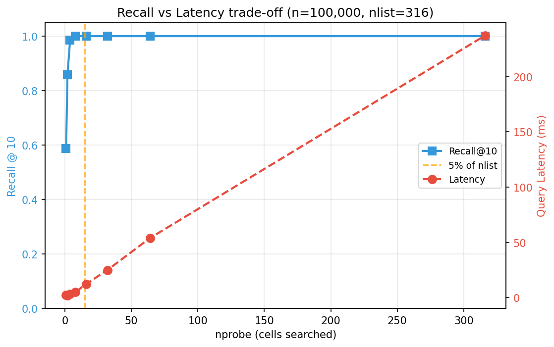

Recall climbs steeply at first (probing just 1.3% of clusters already hits 98.6% recall) and then flatlines while latency keeps growing linearly. Past the knee of the curve, every additional cluster probed costs time without improving results. Finding that optimal value of nprobe is key.

HNSW

Hierarchical Navigable Small World (HNSW) is the gold standard for vector indexing, requiring no pre-training and no centroid count to tune. The implementation follows the original paper.

The name describes the structure:

• Small World: every node connects to its M nearest neighbors, forming a graph where any two nodes are reachable in $O(\log N)$ hops, a property of navigable small-world networks. Higher M means a better-connected graph (better recall, more memory).
• Navigable: search is a greedy walk: at each hop, move to the neighbor closest to the query. The ef parameter controls how many candidates to track during this walk: ef=1 is pure greedy, while higher ef explores more paths for better accuracy.
• Hierarchy: multiple layers stacked on the small world graph: sparse at the top for fast coarse navigation, and dense at the bottom for precision. Each node appears at a random layer drawn from an exponential distribution — most nodes only exist at layer 0, a few reach higher layers.

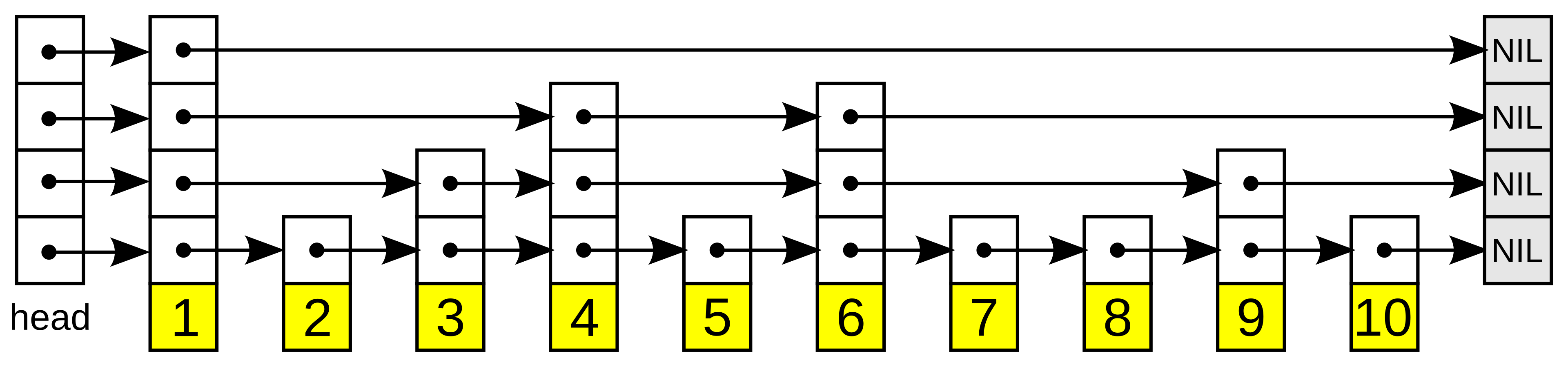
If you’ve seen a skip list, this is the same idea generalised to vectors: express lanes at the top let you take long hops toward the target, then you drop to denser layers for precision. The difference is that a skip list’s “closeness” is a 1D key comparison; HNSW’s is a vector distance.

Search enters at the top layer, greedily descends toward the query, then repeats on each denser layer until layer 0. To power the index, we’ll build a low-level primitive that helps build both indexing and search phase. This is Dijkstra’s algorithm at its core, greedily expanding the closest unvisited node, with one difference: we skip exploring any neighbor that can’t improve on our current ef best results. This bounds the search to a local neighborhood rather than the full graph.

def _search_layer(self, query: np.ndarray, entry_ids: list[int], ef: int, layer: int) -> list:
    # Seed the candidate min-heap with all entry points
    candidates = []  # min-heap: (dist, id): closest node explored next
    for node_id in entry_ids:
        dist = np.linalg.norm(query - self._nodes[node_id].vector)
        heapq.heappush(candidates, (dist, node_id))

    best = []    # max-heap: (dist, id): worst of current top-ef results at front
    visited = set()

    while candidates:
        d, node_id = heapq.heappop(candidates)
        if node_id in visited:
            continue
        visited.add(node_id)

        heapq.heappush_max(best, (d, node_id))
        if len(best) > ef:
            heapq.heappop_max(best)  # evict the furthest if over budget

        for nb_id in self._nodes[node_id].neighbors.get(layer, []):
            nb_dist = np.linalg.norm(query - self._nodes[nb_id].vector)
            if len(best) < ef or nb_dist < best[0][0]:  # only explore if promising
                heapq.heappush(candidates, (nb_dist, nb_id))

    return sorted(best)  # closest first

The index itself holds two things: the nodes (each storing a vector and a per-layer neighbor list), and bookkeeping for the current entry point and top layer. M, ef_construction, and ef_search are the HNSW parameters OpenSearch exposes for tuning.

@dataclass
class HNSWNode:
    vector: np.ndarray
    neighbors: dict[int, list[int]] = field(default_factory=dict)  # layer → [node_ids]


class HNSWIndex:
    def __init__(self, M: int = 16, ef_construction: int = 200, ef_search: int = 50):
        self._M = M                          # max neighbors per node per layer
        self._ef_construction = ef_construction  # beam width during insert
        self._ef_search = ef_search          # beam width during search
        self._nodes: dict[int, HNSWNode] = {}
        self._entry_point: int | None = None
        self._max_layer: int = 0
        self._mL = 1 / np.log(M)            # layer probability scale

    def _random_level(self) -> int:
        # Exponential distribution: most nodes at layer 0, exponentially fewer above
        return int(-np.log(np.random.uniform()) * self._mL)

    def index(self, vector: np.ndarray) -> None:
        node_id = len(self._nodes)
        node = HNSWNode(vector=vector)
        self._nodes[node_id] = node
        node_layer = self._random_level()

        if self._entry_point is None:
            self._entry_point = node_id
            self._max_layer = node_layer
            return

        # Phase 1: ef=1 greedy descent through layers above node_layer: find a close entry point
        entry_ids = [self._entry_point]
        for layer in range(self._max_layer, node_layer, -1):
            entry_ids = [nid for _, nid in self._search_layer(vector, entry_ids, ef=1, layer=layer)]

        # Phase 2: beam search at each layer from node_layer down to 0: wire edges
        for layer in range(min(node_layer, self._max_layer), -1, -1):
            M_limit = self._M * 2 if layer == 0 else self._M
            results = self._search_layer(vector, entry_ids, ef=self._ef_construction, layer=layer)
            entry_ids = [nid for _, nid in results]

            # Connect new node to its M nearest neighbors at this layer
            node.neighbors[layer] = [nid for _, nid in heapq.nsmallest(M_limit, results)]

            # Bidirectional: each neighbor adds a back-edge, then prunes to M
            for nb_id in node.neighbors[layer]:
                nb = self._nodes[nb_id]
                all_edges = nb.neighbors.get(layer, []) + [node_id]
                scored = [(np.linalg.norm(nb.vector - self._nodes[n].vector), n) for n in all_edges]
                nb.neighbors[layer] = [nid for _, nid in heapq.nsmallest(M_limit, scored)]

        if node_layer > self._max_layer:
            self._max_layer = node_layer
            self._entry_point = node_id

    def search(self, query: np.ndarray, k: int) -> list[tuple[int, float]]:
        # ef=1 descent to layer 1: fast coarse navigation
        entry_ids = [self._entry_point]
        for layer in range(self._max_layer, 0, -1):
            entry_ids = [nid for _, nid in self._search_layer(query, entry_ids, ef=1, layer=layer)]
        # Full beam search at layer 0: precision
        return self._search_layer(query, entry_ids, ef=self._ef_search, layer=0)[:k]

HNSW in action: a worked example

Using the same 8 vectors, suppose the graph has been built with M=2 and looks like this at layer 0 (edges connect nearest neighbors):

Layer 1 (sparse):    v3 ——— v5
                       \
                        v0

Layer 0 (dense):     v0 — v1 — v2
                      |         |
                     v6 — v7   v3
                            \   |
                             v4—v5

To search for $q = [5.0, 5.0]$ with k=1:

Phase 1: Layer 1 (ef=1): Start at entry point $v3=[8,9]$. Check its neighbors: $v5=[8.5,8.5]$ (farther), $v0=[1,2]$ (farther). $v3$ is the local best: descend with $v3$ as entry.

Phase 2: Layer 0 (ef=ef_search): Start at $v3$. Expand neighbors $v4, v5, v7$. $v7=[6,2]$ is closer (dist=3.16). Expand $v7$‘s neighbors: $v6=[5,1]$ (dist=4.0), $v4=[9,8]$ (farther). No improvement found: return $v7$ as the nearest.

The greedy descent found $v7$, and it turns out $v7$ is indeed the closest true neighbor (distance is 3.16, compared to $v3$‘s 5.0). The key insight: HNSW only visits a small fraction of nodes. In this toy example it checked 5 of 8 vectors; at scale with a million vectors and M=16, a search typically visits a few hundred nodes.

Tuning HNSW parameters

• M (edges per node): Controls graph connectivity. Higher M means more edges, better recall, but more memory. Each doubling of M roughly doubles the index size. M=16 is a solid default; increase to 32-64 for datasets where recall matters more than memory.

• ef_construction (beam width during index building): How many candidates to consider when connecting a new node. Higher values produce a better-connected graph at the cost of slower indexing. ef_construction=200 is a common default; for large production indexes, 100-500 is typical. This only affects build time, not search.

• ef_search (beam width during query): The runtime accuracy/speed knob, analogous to IVF’s nprobe. Must be $\geq k$. Start at 50 and increase until recall stabilizes. Unlike M and ef_construction, this can be tuned per-query without rebuilding the index.

Benchmarking HNSW

Our pure-Python implementation above is faithful to the paper, but far too slow for realistic benchmarks. Indexing 100k vectors takes minutes instead of seconds. The numbers below use hnswlib, a production-grade C++ implementation of the same algorithm, with the same M, ef_construction, and ef_search parameters. On the same clustered dataset:

> uv run plot_hnsw_performance.py
  n=  1,000 | Flat=    1.54 ms | IVF=  0.51 ms | HNSW=  0.058 ms
  n=  5,000 | Flat=    5.36 ms | IVF=  0.96 ms | HNSW=  0.042 ms
  n= 10,000 | Flat=   12.10 ms | IVF=  1.57 ms | HNSW=  0.046 ms
  n= 25,000 | Flat=   28.73 ms | IVF=  2.46 ms | HNSW=  0.060 ms
  n= 50,000 | Flat=   64.24 ms | IVF=  6.55 ms | HNSW=  0.073 ms
  n=100,000 | Flat=  143.35 ms | IVF= 11.15 ms | HNSW=  0.095 ms

At 100k vectors, HNSW queries take 0.095ms, which is 1500x faster than flat search and 100x faster than IVF. The $O(\log N)$ scaling is visible: latency barely moves as the corpus grows from 1k to 100k.

Sweeping ef_search on the 100k index shows the same recall/latency pattern as IVF’s nprobe:

At ef_search=50, recall is 96.8% at 0.115ms per query. Doubling to ef_search=100 reaches 99.6% at 0.160ms. The full useful range fits within sub-millisecond latency.

The recall trade-off

Every approximate algorithm sacrifices some accuracy for speed. Recall@k measures this: of the true $k$ nearest neighbors, what fraction does the algorithm actually return?

A recall of 0.95 means the algorithm finds 95 of the true 100 nearest neighbors. The remaining 5 are close. They’re near-misses, not random vectors from the other side of the space. For most applications (RAG, recommendations, semantic search), this is indistinguishable from exact search.

The relationship between recall and speed is different for each algorithm:

In practice, HNSW typically achieves 95%+ recall while searching less than 1% of the dataset. IVF can match this recall but needs a well-chosen nlist and nprobe, a training step that HNSW avoids entirely. The flat index remains the right choice for small datasets or when you need guaranteed exact results.

Conclusion

Each algorithm occupies a different point in the accuracy/speed/memory space:

• Flat Index: exact results, no parameters to tune, $O(N \cdot D)$ per query. Use it for $N < 10{,}000$ or as ground truth to validate approximate indexes.
• IVF: requires a k-means training step, but uses no extra memory beyond the centroids. Tune nlist and nprobe to control the accuracy/speed curve. Fits when memory is constrained and you can afford offline training.
• HNSW: no training step, $O(\log N)$ queries, 95%+ recall out of the box. The graph edges add $O(N \cdot M)$ memory on top of the vectors. The default choice when latency matters.

These algorithms are building blocks, not final answers. Production systems combine them: IVF for coarse filtering with product quantization for compression, or HNSW with metadata pre-filtering. The ANN Benchmarks project (ann-benchmarks.com) tracks how these combinations perform across real datasets.